Automatic detection of unwanted noise

A major task in any Data Science project is data cleaning. Without proper cleaning, data can be biased, polluted or even inconsistent. If a machine learning model is fitted using such data, the results obtained are unlikely to be reliable.

In this project, I used machine learning to enhance and speed up the process of cleaning of audio recordings. In these recordings, parasitic noise can occur, but they are not known beforehand. Therefore, developing an unsupervised method is mandatory.

Results​

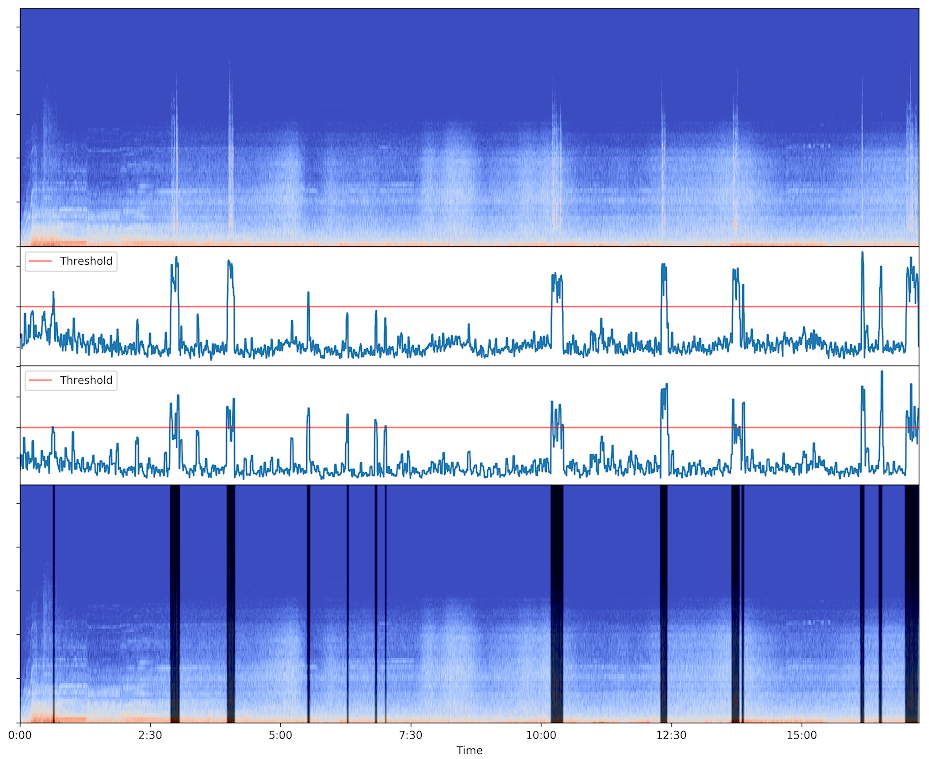Input spectrogram (top) - Anomaly scores (middle) - Ouput spectrogram with dark frames for parts classified as anomalies (bottom)

Pipeline​

1. Harmonic-Percussive Source Separation
2. Extraction of features from the signal
3. Features enrichment with statistical indicators
4. Scoring using a Isolation Forest (unsupervised anomaly detection)
5. Rolling window to smoothen the results

Harmonic-percussive source separation​

A spectrogram is a 3D representation of a signal. Time is usually represented along the x-axis, and frequency along the y-axis. The z-axis corresponds to the amplitude and is conveniently represented using a colormap. The signal is divided into frames, and for each frame is calculated a spectrum (a column of pixels in the spectrogram).

This representation allows human eye to "visualize" the sound.

Horizontal lines correspond to tonal noise (nearly constant frequency), whereas parasitic noises usually span vertically on a spectrogram. It can be shocks, clicks, voice and so on. Using a right sized window, the harmonic-percussive source separation (HPSS [1]) allows to separate and filter out tonal and broadband noise, to keep the percussive component (vertical lines).

Below is an example taken from librosa's documentation on the effect of applying the HPSS on a sample recording.

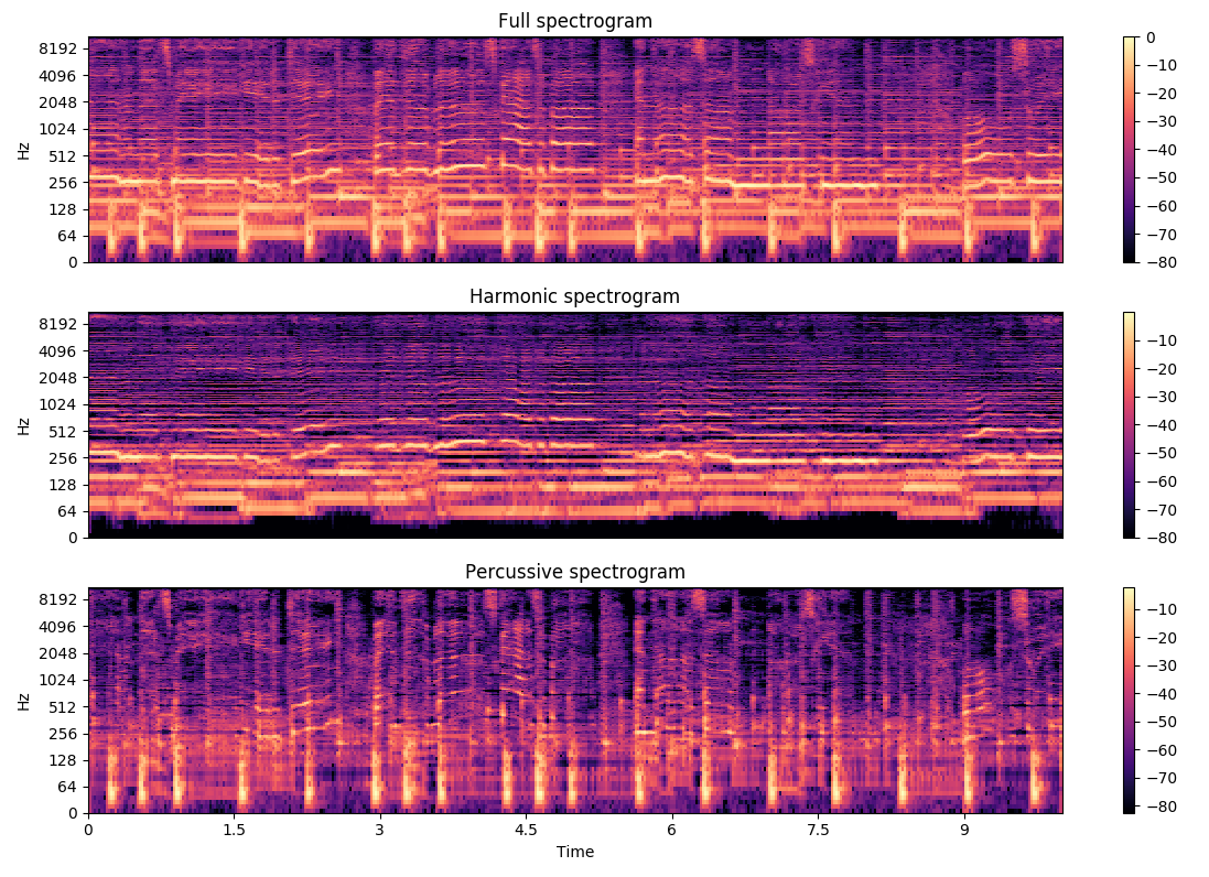Example from librosa documentation

Features extraction​

Several features are extracted from the signal, using the librosa python library [2].

Mel-frequency cepstral coefficients (MFCCs)​

The detection uses 15 MFCCs computed by librosa.feature.mfcc

MFCCs are commonly derived as follows [3]:

1. Divide signal into frames.
2. Take the Fourier transform.
3. Convert to a mel-scale.
4. Take the logs of the powers.
5. Take the discrete cosine transform.
6. The MFCCs are the amplitudes of the resulting spectrum.

Spectral contrast​

The detection uses 6-band spectral contrast [4] computed by librosa.feature.spectral_contrast

Each frame of a spectrogram S is divided into sub-bands. For each sub-band, the energy contrast is estimated by comparing the mean energy in the top quantile (peak energy) to that of the bottom quantile (valley energy). High contrast values generally correspond to clear, narrow-band signals, while low contrast values correspond to broad-band noise.

Zero-crossing rate​

Computed by librosa.feature.zero_crossing_rate. The zero-crossing rate is defined as the rate of sign-changes along a signal.

Spectral Rolloff​

Computed by librosa.feature.spectral_rolloff

The roll-off frequency is defined as the frequency below which a given percentage of the energy of the spectrum is contained.

Onset-strength​

Computed by librosa.onset.onset_strength

Compute a spectral flux onset strength envelope [5].

RMS​

Computed by librosa.feature.rms

Compute the root-mean-square (RMS) value for each frame.

Features enrichment​

To enrich the dataset, we compute for each feature, using a sliding window.

• Corrected sample standard deviation:

  $$s=\sqrt{\frac{1}{N-1}\sum_{i=1}^N(x_i - \bar{x})^2}$$

  where $\bar{x}$ is the sample mean.

  The higher $s$ is, the higher the local dispersion of data.

• Sample skewness:

  $$G_1 = \frac{k_3}{k_2^{3/2}} = \frac{\sqrt{n(n-1)}}{n-2}\frac{\frac{1}{n}\sum_{i=1}^n(x_i-\bar{x})^3}{\left[\frac{1}{n-1}\sum_{i=1}^n(x_i-\bar{x})^2\right]^{3/2}}$$

  where $\bar{x}$ is the sample mean.

  The higher the absolute value of $G_1$, the more asymmetric the distribution of data.

• Sample kurtosis:

  $$g_2 = \frac{m_4}{m_2^2}-3 = \frac{\frac{1}{n}\sum_{i=1}^n(x_i-\bar{x})^4}{\left[\frac{1}{n}\sum_{i=1}^n(x_i-\bar{x})^2\right]^2}$$

  where $\bar{x}$ is the sample mean.

  The higher $g_2$ is, the fatter the tails of the distribution, hence, the higher the number of extreme values.

Isolation Forest​

The main approaches when it comes to detecting anomalies consists in profiling what a normal point is. Isolation Forest [6] uses a completely different method. Instead of focusing on normal points, it isolates the abnormal ones.

When we see a lineplot (1D), we can easily imagine setting a range of acceptable values. However, this range may change along a second dimension. For example, what can be considered as normal for a temperature of 20°C may not be at 50°C. The Isolation Forest method has the ability to work with n-dimension data.

An Isolation Forest is composed of multiple trees

The algorithm to build a tree is the following:

1. Take a sample of the dataset

2. Select a random attribute (dimension)

3. Select a random split point for this attribute

4. Split the sample (using the split point) into two subsets.

5. Repeat steps 2 to 4 for each of the two subsets, until the maximum depth is reached.

By creating trees using random attributes, we ensure that all the trees in the forest will be different.

After generating a given number of trees, we can compute for each point $x$ the average path length $h(x)$ from the roots. A point considered abnormal is easier to isolate, and will have a lower average path length.

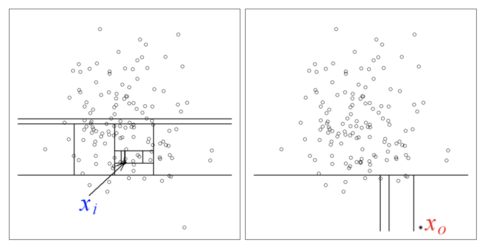$x_i$ can be considered as normal, $x_0$ as an anomaly

A score $s$ is calculated for each point $x$ using:

• the average path length in all trees $E(h(x))$,
• the average path length of unsuccessful search in a Binary Search Tree $c(n)$ where n is the sample size

The scores given to the points have the following meaning:

• When $s$ is close to 1, $x$ is very likely to be an anomaly.
• When $s$ is much smaller than 0.5, $x$ can be considered as normal.

Finally, to reduce the possibility of false-positive (points labeled abnormal instead of normal), a rolling windows can be apply to smoothen the results (n-decile, standard-deviation etc).

References​