TGV economic performance optimization
Dynamic Programming
Dynamic programming is an optimization method based on breaking down a big problem into smaller problems that are easier to solve.
In this project, the main benefits of using dynamic programming are the following:
- We don't know a priori what the shape of the solution would be, but we can formalize the problem, its constraints, and the metrics to be optimized.
- We can explore possible ways to operate the train, and keep track of the previous states of the search: we don't have to start from the beginning each time we run into a dead-end.
- We can generate more than one solution, and therefore explore trade-offs between energy savings and delay.
Therefore, we can think of dynamic programming as smart brute-force method. At each iteration we explore a most-promising node, and cut out the ones that are already breaking a constraint.
For instance, if we were to truly brute-force a 100-step problem with 5 possibilities for each node, we would have to generate an unthinkable number of paths:
However, if the constraints we have set are actually restricting possibilities to an average of 1.1 possibilities for each node, we restrict the research space to:
It was a brief introduction to dynamic programming, but hopefully you will get the intuition behind why it works.
Optimization of the train operation
When it comes to optimizing the energy consumption of a train, we can breakdown the whole trip from point A to point B into shorter segments. Instead of optimizing a 100km trip directly, we can start by optimizing the first kilometer. The problem can be represented as a graph with a root node being the origin station, and a terminal node being the next station to reach. Nodes in between will be steps allowing to reach our goal (the terminal node).
A node consists of:
- Current speed: the speed at which the train will operate for the next segment.
- List of previous speeds: to keep track of the operation history.
- Trip duration: since departure from the root node.
- Traveled distance: from the root node.
- Consumed energy: this one metrics to be optimized compared to a reference.
After each segment, there will be a decision-making step: do we accelerate, decelerate or keep constant speed ?
Initialization of the problem
We start the optimization by generating the root node: all the properties of the node will be equal to zero. Then we generate children nodes based on reachable speeds within the next segment; with regards to laws of physics, and external constraints (maximum speed for instance).
Main loop
Until we reach the terminal node (or when paths are found), we will proceed as follows:
- Select the node with the best heuristic that we define (it can be the best delay to energy saved ratio)
- Generate a child for each reachable speed within the next segment, if all the constraints are still respected. Each child will have a different current speed, trip duration and consumed energy, but a common list of previous speeds as they are generated from the same parent.
Solutions
We can either decide to end the search:
- as soon as we have found a solution
- as soon as we generated paths from the root node to the terminal node
The first one will indeed be the fastest option, but the second one will allow to get a set of different paths, having different delays and energy savings. From this set we can identify a pareto front of paths achieving best trade-offs.
Results
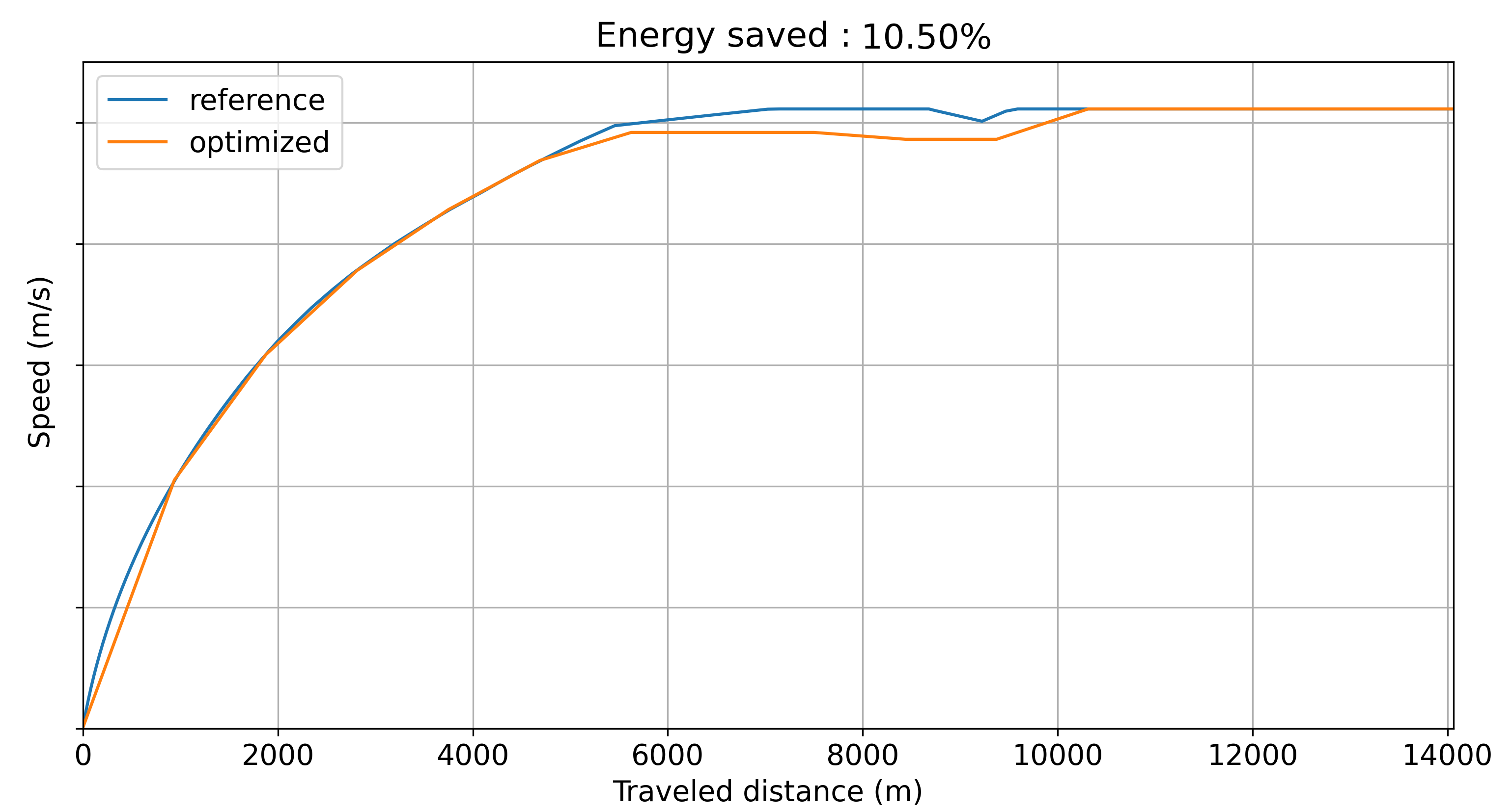 Optimized speed curve
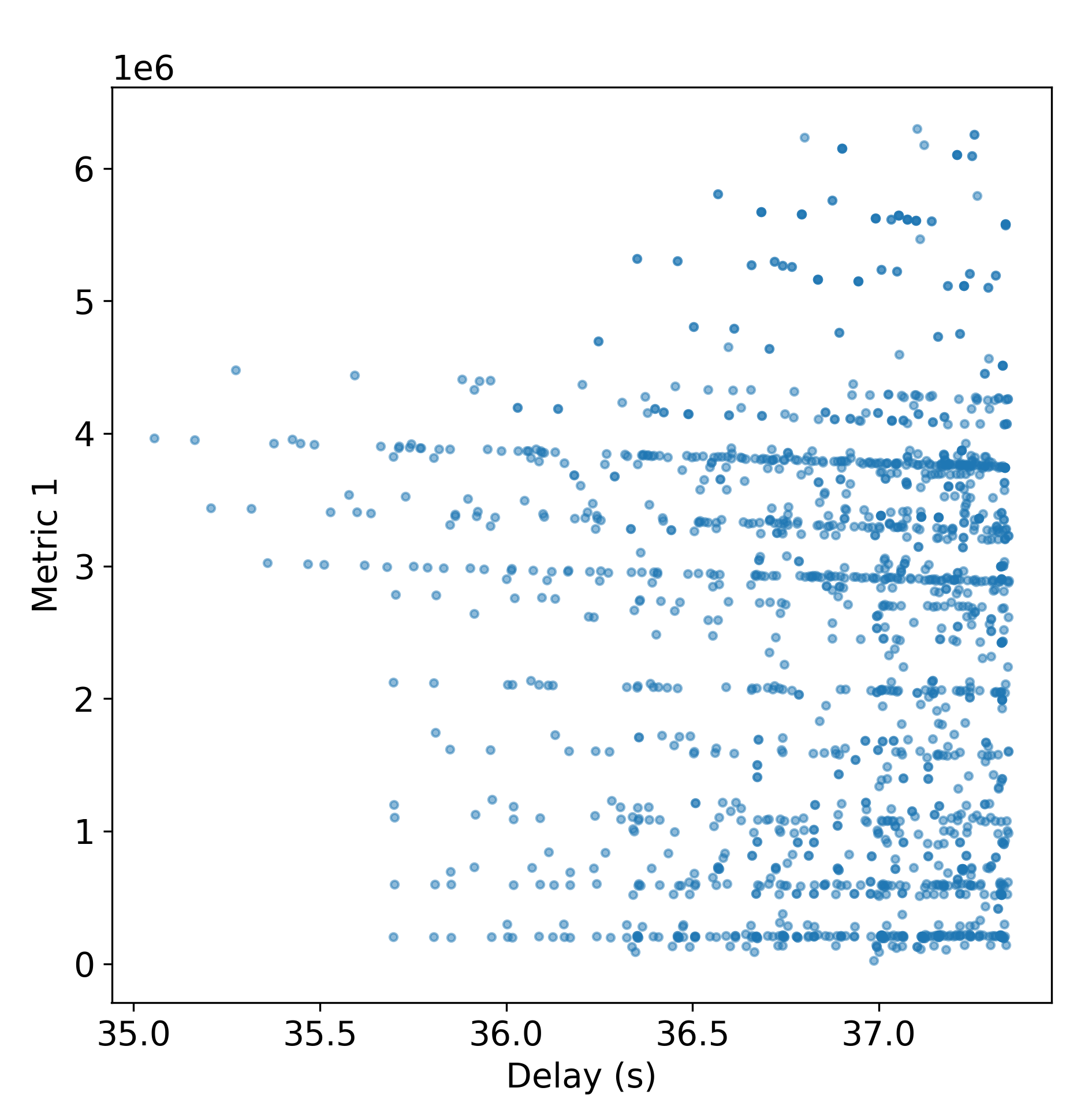 One of the metrics tested (top left is better)